


Big O Notation — The Intuition Behind
Understand the basics of time complexity analysis!

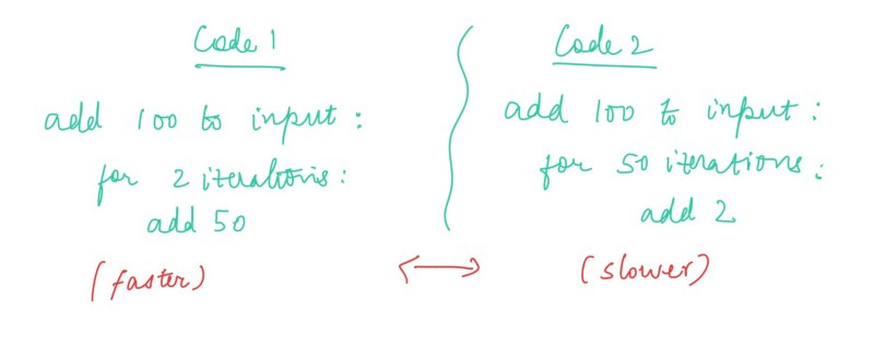
When we look at two pieces of code, we can somehow see and tell which one is gonna be relatively faster and which one is gonna be relatively slower — But the Big O Notation gives us the power to determine that definitively.
Big O is the metric used to describe the efficiency of algorithms.
So what does the ’n’ in O(n) mean?
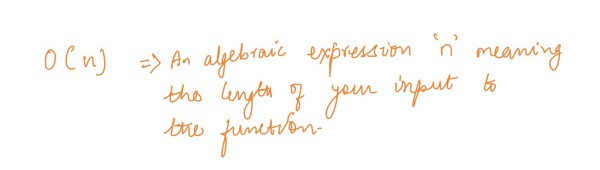
Yep! ’n’ is simply the length of the input you provide to your function. The function can consist of anything and with Big O notation, we can express its runtime in terms of — how quickly it grows or shrinks relative to the input you provide, as the input gets arbitrarily large or small.
Let us run through one small piece of real life example and try to “decode” its time complexity by understanding it:
Imagine the scenario: You need to send a file from your computer to someone who needs it, ten thousand kilometres away. What should be the best possible method to send it?
Now, before you think about a method such as FTP(File Transfer Protocol) or even something like email, you need to consider how big the file actually is.
Thus, for sending a 1 Terabyte file, it will be faster to send it over by a plane physically than try to send it via electronic means, which might take a day or even more than only a few hours via the plane.
Here’s the moment when the concept of Time Complexity with the Big O notation comes into play.
If you send the file via email, it’ll most likely be of time O(n): where n will be the length of the file.
If you send it via a plane, it’ll be a constant time — why? Because delivering the file with a plane will not depend on the size of the file. Even if the size is a little more or a lot more, the plane will take the same amount of time to deliver it.
Thus, you can now see that we use Big O notation to talk about how quickly the runtime grows practically, and how our input influences that growth.
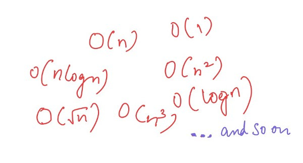
Different forms of Big O
Now, as you might have already guessed, O(n) can be of many forms: the algebraic notations can be written as one of many kinds as shown.
Let’s now look at a piece of pseudocode and get some idea of what calculating this might actually look like in the form of a pseudocode.
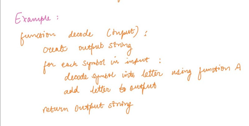
Consider this example: you are decoding a string consisting of symbols for a friend and outputting a string made of letters. You decode these symbols into individual letters using some function A.
Now, looking closely at each of the lines:
creating and returning the output string each needs to happen only once, so take constant 2 as the time for the both of them together.
since we’re going to run the loop on each symbol — one by one — of the input string, we can say that the two lines of code inside the for loop will run 2n times.
Hence, we get the time complexity as: O(2n)
But in practise, we write it as O(n) simply, disregarding the constant terms in the face of the linear terms.
Here, the main point to note is that the each of the two lines of code inside the for loop will take only O(1) time each.
Thus, we might need additional time if function A which we’re using to decipher the symbols into letters takes more than O(1) time. If time taken, for example, is O(n) for function A, then the overall time complexity will become the second order of n, or O(n²) for the decode function!
The Math is Important!
You guessed it right, the math behind this time complexity notation is something you’ll also need to grasp to have a better understanding. Now that we have already looked at a real life example and a small snippet of pseudocode to know what is happening behind the scenes, let’s learn the concept of some concrete math behind it too.
If you’re reading this, you might already know about the popular sorting algorithm called Bubble Sort.
Bubble Sort has the time complexity in the worst case as O(n²). Let us try to visualise the math behind the complexity and try to understand how exactly it came to be.
Look at the code first!
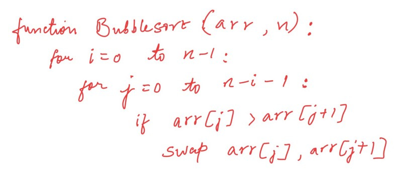
To simplify, here are the steps in the algorithm(for sorting a given array in ascending order):
Starting with the first element(index = 0), compare the current element with the next element.
If the current element is greater than the next element of the array, swap them.
If the current element is less than the next element, move to the next element. Repeat Step 1.
The code contains two nested loops running through basically all the elements of the array and comparing them again and again.
Study this worked out example:
Taking an array of length 5 and elements = {5, 1, 8, 2, 4}, we can try out the Bubble Sort algorithm by hand like this:
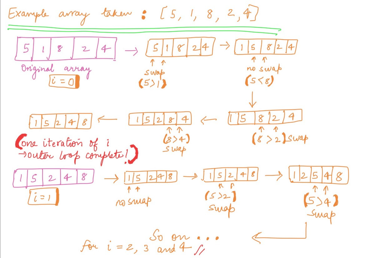
Now, you might be wondering why we will be considering the i=2,3 and 4 iterations when the array becomes fully sorted in ascending order only after i=0th and 1st iteration.
Here’s the answer: Bubble sort is designed to compare each element by its adjacent element for the whole length of the array — thus, for i = 0, it’ll compare the elements from j=0 to j=n — i — 1 = 5–0–1 = 4 times!
Therefore, the loop will keep running for all 5 iterations even after the sorting is done.
Hence, we can certainly agree, even without the math behind it yet that this sorting algorithm is not very efficient!
Now, we’ll look at its time complexity.
Warning: Some jargon ahead! :)
To calculate the complexity of the Bubble sort algorithm, it is useful to determine how many comparisons each loop performs(we have two of them nested!).
Let’s look at the comparisons we did when we worked out the algorithm by hand. For each element in the array, it does n−1 comparisons. In Big O notation, Bubble sort performs O(n) comparisons.
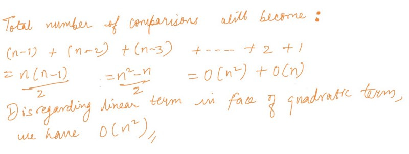
So, n — 1 comparisons will be done in the 1st iteration, n — 2 in the 2nd , n — 3 in the 3rd and so on. In other words, it will perform O(n) operations on an O(n) number of elements, leading to a total running time of O(n²).
But when does this n² running time actually come into effect, you might ask.
Different kinds of time complexity along with how good and how bad they are in practise.
Now that we have looked at a real algorithm and its time complexity with Big O notation, we can look at how different forms of Big O compare with each other in terms of runtime, because that is what we’re really concerned with and hoping to, eh, optimise for our code, aren’t we?
Alright, runtime it is!

I hope that with this, you might have come to an understanding of exactly what the Big O notation entails and can now go into reading further and practise it on real coding problems to become better at it. :)
For recommended reading resources, I’ll highly suggest you to go read these:
Cracking The Coding Interview Book, from Gayle Laakmann, the most thorough guide on all kinds of coding interview problems, along with a good portion of the book dedicated to algorithms, data structures and time complexity analysis too(from which a snippet of this article is also inspired).
The Big O Algorithm Complexity Cheat Sheet which has a clean, easy to understand list of all Big O algorithms and how different data structures associate with them in different operations like Insert, Delete, Access etc, all in one page!
Thank you for reading, and if you liked this article, please be sure to leave a few claps to show your appreciation! ❤